Original paper
Communication-Efficient Learning of Deep Networks from Decentralized Data
- Publication
- AISTATS 2017Conference
- First submitted to arXiv
- arXiv:1602.05629
Cite this paper · BibTeX
The citation identifies the linked source version. It cites the original paper and its authors.
@misc{modelmergingfedavg2016,
  title = {{Communication-Efficient Learning of Deep Networks from Decentralized Data}},
  author = {H. Brendan McMahan and Eider Moore and Daniel Ramage and Seth Hampson and Blaise Agüera y Arcas},
  year = {2016},
  eprint = {1602.05629},
  archivePrefix = {arXiv},
  url = {https://arxiv.org/abs/1602.05629}
}
For next-word prediction on a phone keyboard, the best training data is what users type every day.
The trouble is that this text includes messages, URLs, even passwords. Uploading all of it to a data center for training carries a large privacy risk. Chat language is also very different from Wikipedia, so a public corpus used as a substitute cannot teach a model how users actually type.
In 2016, McMahan, Moore, Ramage and colleagues at Google proposed keeping the data on the phone, with each phone sending the server only “how the model should change.” They called this approach federated learning and gave a very plain algorithm for it, FederatedAveraging, which everyone later shortened to FedAvg.
The paper also matters in the context of model merging. Round after round, FedAvg repeats one operation, directly averaging many separately trained copies of the weights. The paper contains a small figure explaining why this works for neural networks, and later model-merging research keeps coming back to that condition.
Defining the problem
Suppose there are clients (phones, for example). Client holds examples, in total. We want to minimize the average loss over all the data:
is the average loss on client 's own data. If the data were randomly shuffled before being distributed, the expectation of every would equal . This is the IID case that standard distributed training assumes.
The authors point out four ways federated learning differs from a data center:
- Non-IID: each phone's data comes from a single user, with a distribution very different from the population as a whole.
- Unbalanced: some people type thousands of words a day; others use the keyboard once a month.
- Massively distributed: the number of participating clients can exceed the average number of examples per client.
- Limited communication: phones are often offline, upload bandwidth is usually below 1 MB/s, and phones are willing to participate only while charging and connected to unmetered Wi-Fi, so each can join only a few rounds a day.
The last point determines how the whole paper measures progress. Computation on the phone is relatively cheap; communication rounds are expensive. When comparing methods, the paper therefore looks at how many communication rounds it takes to reach a target accuracy.
The goal is to spend a bit more local computation in exchange for fewer communication rounds. There is a big problem, though. Neural network losses are nonconvex, so directly averaging two separately trained sets of weights could, in theory, produce a terrible model. Why should averaging work?
Solving the problem
Starting from FedSGD
The authors first define a baseline. Each round randomly selects a fraction of the clients. Each selected client computes the gradient over all its data, , and the server updates with the gradients averaged by data size:
This is large-batch synchronous SGD, which the paper calls FederatedSGD (FedSGD). controls the global batch size of each round; is full-batch gradient descent.
The authors then rewrite the same update. Each client first takes one step with its own gradient, and the server then averages the weights:
The two forms are mathematically equivalent. Every client starts from the same , so averaging the weights is the same as averaging the gradients.
Once the update is written in the second form, the next step comes naturally. If each client already takes one local step, why not take several before reporting back?
FedAvg
FedAvg has each client run several passes of SGD locally, then send its weights back to the server for averaging. Three parameters control the amount of computation:
- : the fraction of clients participating in each round.
- : how many epochs each client runs over its local data.
- : the local minibatch size; means the whole local dataset is treated as one batch.
A client with examples performs local updates per round. With and , FedAvg reduces to FedSGD.
Written as code, the server side looks roughly like this:
def fedavg_round(w, clients, C, E, B, lr):
    m = max(int(C * len(clients)), 1)
    selected = random.sample(clients, m)
    total = sum(c.num_examples for c in selected)

    new_w = zeros_like(w)
    for c in selected:
        w_k = client_update(c, w, E, B, lr)          # start from the same w, run E local epochs
        new_w += (c.num_examples / total) * w_k      # weight by the data size of this round's participants
    return new_w
The denominator of the weighted average is the total data held by the clients selected this round, . Suppose this round picks three phones with 600, 300 and 100 examples. Their weights are then 0.6, 0.3 and 0.1, and a client with more data has more influence on the new model.
Why averaging works
Back to the earlier question. The authors answer it with a small experiment.
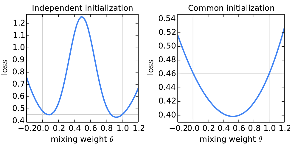
The setup is small. Two multilayer perceptrons, and , are each trained on a non-overlapping set of 600 MNIST examples, with learning rate 0.1 and batch size 50 for 240 steps (equivalent to 20 epochs), roughly to the point where they begin to overfit their local data. The authors then compute the loss of on the full training set, sweeping from −0.2 to 1.2.
Look at the left plot first. The two models are initialized with different random seeds. Both endpoints have a loss of around 0.45, but the averaged model in the middle shoots above 1.2, worse than either one.
Now the right plot. The two models start from the same random initialization, and the curve becomes a bowl. The loss of is about 0.40, clearly below the roughly 0.46 loss of each parent model. Note that the two plots use different vertical scales; the entire right-hand curve is low.
In every round of FedAvg, all clients start from the same , which is exactly the situation in the right plot. The authors do not prove that this holds for all networks. They only cite observations made at the time about the loss landscapes of overparameterized networks, then use this figure to illustrate the intuition.
The idea that “weights from a common starting point can be averaged directly” later recurs throughout model-merging work such as SWA, Model Soups and task arithmetic, and there, too, the condition is a shared starting point.
Discussion
Experimental setup
The authors trained more than two thousand models across five model types and four datasets:
- MNIST 2NN: a multilayer perceptron with two layers of 200 units each, 199,210 parameters.
- MNIST CNN: two 5×5 convolutional layers plus a 512-unit fully connected layer, 1,663,370 parameters.
- Shakespeare LSTM: a character-level two-layer LSTM, 866,578 parameters.
- CIFAR-10: the small CNN from the TensorFlow tutorial, about parameters.
- Large-scale next-word prediction LSTM: a 10,000-word vocabulary, 4,950,544 parameters.
How the data is partitioned is the heart of this paper. For the IID version of MNIST, the data is shuffled and distributed to 100 clients with 600 examples each. The non-IID version first sorts the data by digit label and cuts it into 200 shards of 300 examples, giving each client two shards. Most clients see only two digits, an extreme case the authors designed on purpose.
Shakespeare is closer to real conditions. The authors treat each speaking role in each play of Shakespeare's complete works as one client, 1,146 in total. Roles with many lines differ greatly from roles with only a few, so the data is naturally both unbalanced and non-IID.
Every setting is swept over a grid of learning rates. The authors take the best learning rate, then count how many rounds the learning curve takes to cross the target accuracy.
Parallelism: how many clients to bring in
The first set of experiments fixes and varies , the fraction of clients participating per round. Take the 2NN with . On IID data, going from 1 client per round to (10 clients) cuts the rounds needed to reach 97% accuracy from 316 to 87; on non-IID data, from 3,275 to 664.
With , increasing helps much less. The authors settle on as the default for later experiments, considering it a good balance between computational efficiency and convergence speed.
A few more local steps
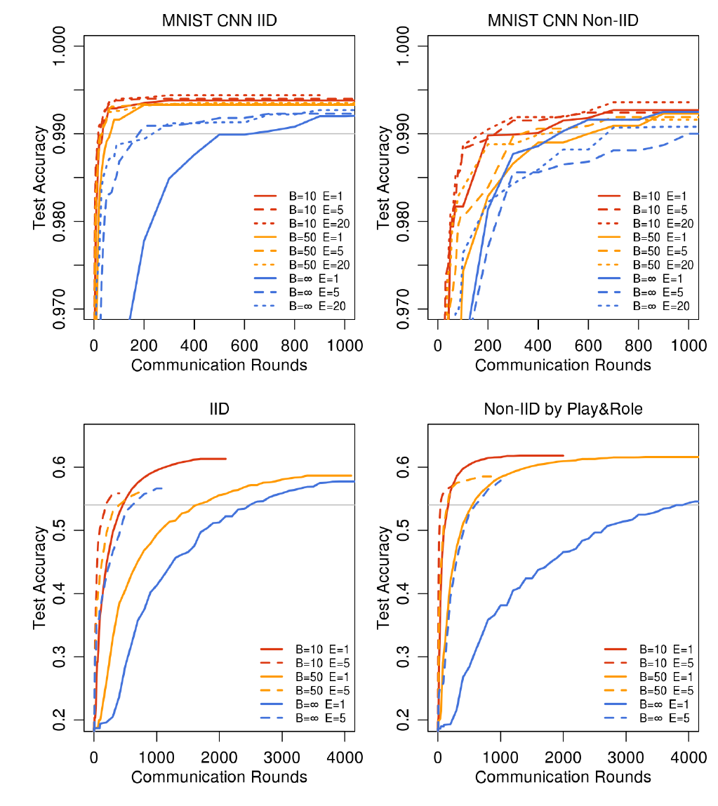
In this figure, watch the distance between the solid blue line and the red lines. The solid blue line is , , which is FedSGD; the red lines are , with the most local updates per round. In all four plots, the red lines cross the gray target line much earlier than the solid blue line.
Converted into the communication rounds needed to reach the target accuracy, FedAvg is several times faster in all four settings.
- MNIST CNN, IID: FedSGD needs 626 rounds to reach 99%; , needs only 18, 34.8 times faster.
- MNIST CNN, pathological non-IID: FedSGD needs 483 rounds, the best setting 173, 2.8 times faster.
- Shakespeare, IID: FedSGD needs 2,488 rounds to reach 54%; , needs 192, 13.0 times faster.
- Shakespeare, split by role: FedSGD needs 3,906 rounds; the same setting needs only 41, 95.3 times faster.
The second item deserves a pause. Each client has only two digits, so the separately trained models differ a lot, yet averaging them is still faster than FedSGD. The authors themselves say it is already surprising that averaging brings any benefit at all instead of simply diverging. Still, the speedup is only about 2.8 times, and some settings in the table are even slower than FedSGD; for example, , takes 1,000 rounds on non-IID data.
The fourth item is a surprise in the other direction. The data split by role gives a larger speedup than the IID version. The authors speculate that some roles have a great many lines, which makes extra local training steps especially valuable. This is speculation; the paper does not verify it further.
Beyond the round counts, FedAvg also reaches higher final accuracy. FedSGD on the MNIST CNN reaches 99.22% after 1,200 rounds and makes no further progress even after 6,000; FedAvg with , reaches 99.44% within 300 rounds. The authors speculate that model averaging has a regularizing effect similar to dropout, and again give no experiment to verify it.
What happens with too much local computation
The larger is, the closer each local model gets to the optimum for its own data. If the problem were convex, the starting point would stop mattering as , and more rounds of averaging would bring no further improvement.
The authors also push very high on the Shakespeare LSTM (up to 200). When is too large, the training loss stalls or even diverges. The MNIST CNN shows no obvious degradation, and on the large next-word prediction task, is slightly better than . The authors therefore suggest cutting the local computation per round late in training, much like decaying the learning rate.
This is the part of FedAvg people question most often. Each client heads in its own direction, and the farther they go, the more likely the average is to drift away from the global objective.
CIFAR-10 and real-world scale
On CIFAR-10, the authors split the 50,000 training images evenly among 100 clients, a balanced IID setting. Another baseline skips partitioning altogether and runs standard SGD with batch size 100.
Counting rounds to reach 80% accuracy, SGD needs 18,000 updates (in the federated setting, each one counts as a communication round), FedSGD needs 3,750 rounds, and FedAvg only 280. For the 85% target, SGD needs 99,000 updates, FedAvg 2,000 rounds, and FedSGD did not reach it within the time the experiments ran.
The last set is next-word prediction at real-world scale. The authors group ten million public social-network posts by author, which yields more than 500,000 clients, with 200 clients participating per round; FedAvg uses , . FedSGD needs 820 rounds to reach 10.5% accuracy, while FedAvg needs only 35, a 23-fold reduction. FedAvg's accuracy also fluctuates less from one evaluation round to the next.
What this paper leaves open
All of these experiments are simulations. The set of clients is fixed, every round is synchronous, and there are no dropouts or malicious updates; the authors rule these practical issues out of scope at the start. The metric is communication rounds; wall-clock time and phone battery drain are not measured directly.
Convergence is also supported only by experiments. The speedup on pathological non-IID data is clearly smaller, and later research took this problem apart more carefully. Zhao et al.'s Federated Learning with Non-IID Data found that under an extreme split where each client has only one class, accuracy can drop by as much as 55%, and attributed the cause to divergence between the local weights and the global weights. SCAFFOLD calls the same phenomenon client drift and corrects local updates with control variates. Li et al.'s convergence analysis shows, under strong convexity and smoothness assumptions, that the learning rate has to decay in the non-IID case.
On privacy, the paper's claims are that “data never leaves the device” and that “only the minimal necessary update is transmitted.” It gives no formal guarantee from differential privacy or secure aggregation; the authors list both as future work.
Conclusion
The FedAvg algorithm fits in half a page. Clients start from the same weights and run a few more passes of local SGD, and the server averages the results weighted by data size. In return, communication rounds drop by one to two orders of magnitude, and there is experimental evidence that training still works on non-IID data.
Google did go on to use it for next-word prediction in Gboard.
Looking back from model merging, the most intriguing part is still that small experiment mixing two sets of weights. Two independently initialized models break the moment they are averaged, while two models that start from the same point get better after averaging. That condition runs through the weight-averaging research of the years that followed.
If you want to try it yourself, the paper suggests tuning first. As long as the batch still keeps the phone's parallel hardware busy, making it smaller costs almost no extra time. Don't get greedy with , though. Run too long locally and every phone pulls the model toward its own data.