Social sites guess whom you might know; shopping sites guess what you might like. Often the same intuition lies behind both: birds of a feather flock together, and you probably like what your friends like.
A Graph Convolutional Network (GCN) turns this intuition into mathematics.
We will start from zero. No graph-theory background is needed; arithmetic is enough, and matrix multiplication will be explained when it appears. By the end, you will have worked through one GCN layer and watched a small model infer other people's answers from just two known ones. Three interactive diagrams let you click and drag your way through the ideas, often faster than reading formulas alone.
Start with a Problem
There are six people. Alice, Bob and Carol are friends with one another, as are Dave, Eve and Frank. Carol and Dave also know each other, providing the only link between the groups.
We know only two things: Alice likes ball games, Frank does not.
What about the other four?
You might guess like this. Bob's friends are Alice and Carol. Alice likes ball games, so Bob may too. Eve's friends are Dave and Frank. Frank does not, so Eve probably does not either.
Guessing from friends is graph convolution's starting point. Step by step, we will turn it into something a computer can calculate.
Graphs: Nodes and Edges
First, a term: a graph is a structure made of just two things:
- Nodes: the objects being described, here six people.
- Edges: relationships between them, here friendships.
A node can also carry numbers describing itself, called features. Here each person has one: how much they like ball games. Alice is 1, Frank 0. For the four unknown people, start at 0.5, halfway between.
A computer cannot see the drawn lines, so we record friendships in a table called an adjacency matrix.
For six people, this is a 6×6 table . Entry in row , column means people and are friends; otherwise it is 0.
Carol's row has 1s under Alice, Bob and Dave: three friends. The number of 1s in a row is the person's friend count, called their degree.
Friendship is mutual, so ; the table is symmetric across its diagonal.
The Obvious Approach: Ask Your Friends
The simplest guess replaces everyone's number with their friends' average.
Bob's friends are Alice (1) and Carol (0.5), averaging 0.75, so he probably likes ball games. Eve's are Dave (0.5) and Frank (0), averaging 0.25, so she probably does not.
A matrix calculates this for everyone at once. Divide each adjacency row by that person's friend count, giving every friend a share, then multiply by how much each person likes ball games (Alice 1, Frank 0, and 0.5 for everyone we don't know). Result multiplies each share in row by the corresponding value and sums them: person 's friends' average. For the six people, that gives 0.5, 0.75, 0.67, 0.33, 0.25 and 0.5.
Bob is 0.75 and Eve 0.25, matching our intuition. But look at Alice and Frank.
The only two people whose answers we knew both become 0.5. Asking only friends throws away what they know themselves.
Two Fixes
Give Yourself a Vote Too
The fix is direct: include self in the average. Add 1s on the adjacency diagonal, giving everyone an extra “self” friend. These are self-loops, , where is the identity matrix, with diagonal 1s and zeros elsewhere.
Alice's new value is , preserving most of her own answer.
More Friends, Less Weight per Vote
An ordinary average gives every friend the same share. GCN adjusts the share using both people's friend counts. Person receives from person :
is the degree after self-loops: friend count plus 1.
Take Bob, whose is 3. Alice () contributes ; Carol () contributes . Carol knows more people, so her voice is shared more widely and reaches Bob a little more quietly.
These shares are symmetric: Bob takes as much from Carol as Carol takes from Bob. In matrix form, this is GCN's , dividing by square-root degrees on both sides. With self-loops, the six degrees are 3, 3, 4, 4, 3 and 3; recomputing with gives new values of 0.64, 0.64, 0.68, 0.39, 0.31 and 0.31.
The left three people are all above 0.5, the right three below, and Alice still leans toward liking ball games. Shares need not sum exactly to 1: Carol's row sums to 1.08, though close.
Why not use ordinary averaging? Both approaches are used. GCN chooses symmetry partly because its spectral derivation simplifies to this form, and partly for numerical stability across layers, preventing values from growing with each multiplication.
Click anyone in the diagram below to see who contributes and how much. Try all three rules, especially what happens to Alice under “Friends only.”
Bob’s new numberGCN weights
- Alice1.00 × 0.330.33
- Self0.50 × 0.330.17
- Carol0.50 × 0.290.14
Sum0.64
That Is One GCN Layer
Writing what we just did on one line gives the GCN paper's formula:
Its three parts each do one job:
- : everyone takes the weighted average of friends and self using those shares. holds everyone's features, one person per row. At the first layer, is the original features, written .
- Multiply by : people often have more than one feature. recombines them into new descriptions, each a weighted sum of old features. It contains the model's learned parameters and is shared by everyone.
- : a nonlinearity. GCN uses ReLU, making negative values 0 and keeping positive values unchanged.
Add another feature: how much each person likes reading. Alice is 0, Frank 1 and everyone else 0.5. For now we choose : the first new feature is ball games minus reading, the second reading minus ball games. After one GCN layer, Alice, Bob and Carol get [0.33, 0], [0.33, 0] and [0.29, 0], while Dave, Eve and Frank get [0, 0.29], [0, 0.33] and [0, 0.33].
The left three people have positive first features; the right three have positive second features. One GCN layer has separated the groups into different features.
During real training, data determines rather than us. We will get to that shortly.
Why Call It Convolution?
If you know image convolutional neural networks (CNNs), this may look familiar.
Image convolution makes each pixel's new value a weighted sum of itself and 8 surrounding pixels, sliding the same weights across the image. Graph convolution similarly makes each node's new value a weighted sum of self and neighbors, sharing across nodes. They perform the same kind of operation, hence graph “convolution.”
The difference lies in neighbors. Pixels have 8 fixed neighbors at upper left, above, upper right and so on, each position with its own weight. Graph neighborhoods vary in size and lack directions, so GCN determines shares only from degrees. This difference seeds much later research; the first stop in Graph Convolutions in the Grand View Garden starts here.
Two Layers See Farther
One layer lets everyone hear their friends. Feed its result into another and they hear friends of friends.
Alice's information reaches Bob and Carol after one layer, crosses the bridge to Dave after two, and reaches Eve and Frank after three. Stacking layers sees people within hops.
Try dragging the slider below.
At the start, only Alice and Frank have answers.
People reached by Alice’s information0 / 5
Dashed rings mark everyone within reach.
Initially, the maximum–minimum gap is 1.00. After one layer the groups are already separated, with a gap of 0.37; after 8 layers it is only 0.18. More layers make everyone's numbers alike until the groups become indistinguishable: over-smoothing. GCN's main experiments use only two layers; deeper appendix experiments peak at two or three.
Let the Model Learn
So far, we supplied the values and . A real GCN must learn.
Make the problem purer. The model knows nothing about ball-game preferences. Each person's only feature is identity; the sole clues are friendships and two answers: Alice likes ball games, Frank does not.
The model smooths twice with , then applies a linear classifier, with softmax turning the two class scores into probabilities that add up to 1, to output each person's probability of liking ball games. Training computes error only from Alice and Frank and adjusts the classifier's weights step by step with gradient descent. With the graph, Bob and Carol are predicted to like ball games (0.98 and 0.92), Dave and Eve not to (0.08 and 0.02): all four correct. Without it, the model knows nothing about them and stays at 0.5.
There are only two answers; everything else follows from friendships. This is GCN's most common use, semi-supervised node classification. On the Cora citation network, the paper supplies classes for only 140 of 2,708 papers; a two-layer GCN predicts the others at 81.5% accuracy.
Watch training step by step below, or switch to “Without the graph” to compare.
Of the 4 people without answers, 0 are on the right side.
How Does It Differ from a Transformer?
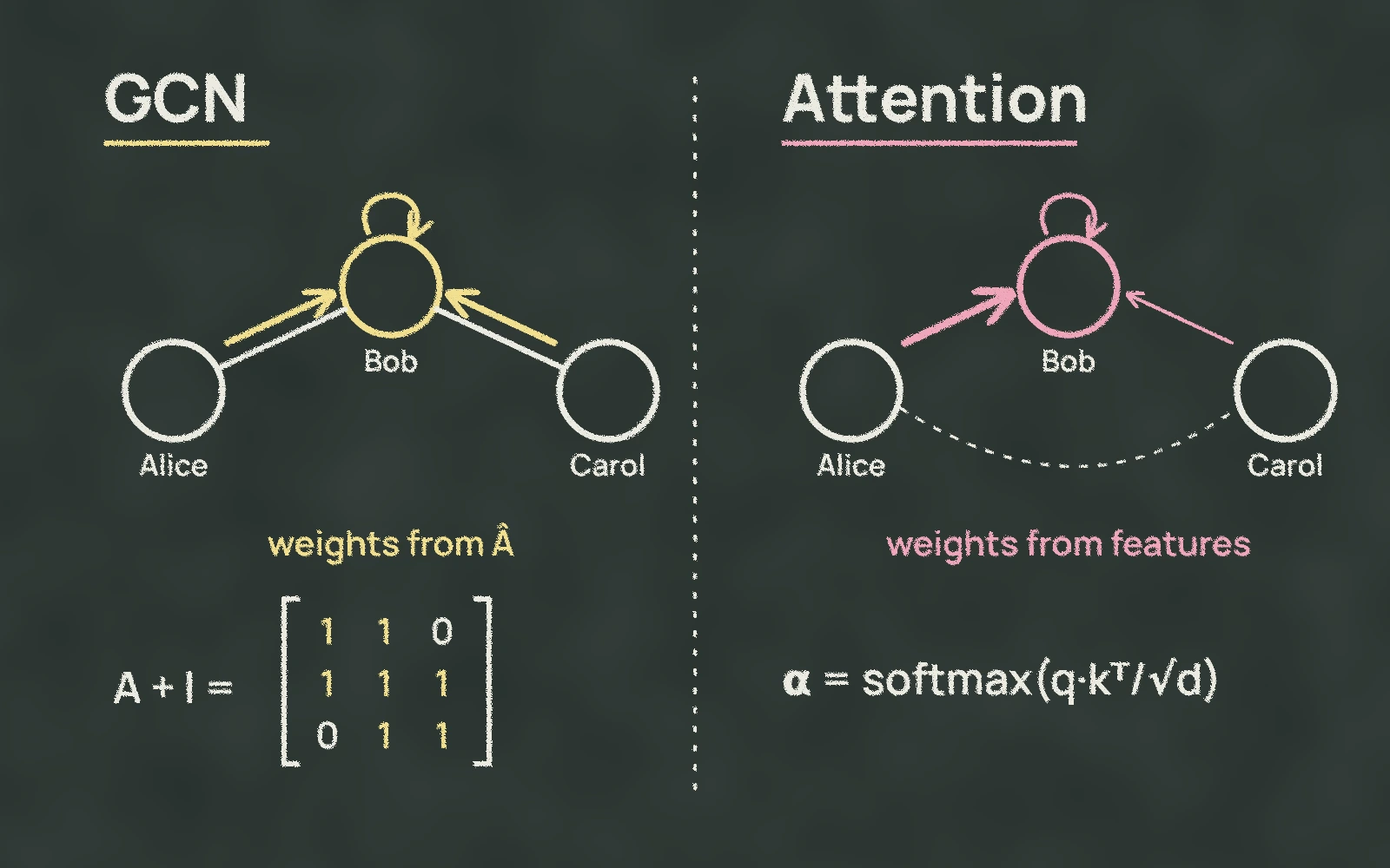
If you know Transformers, taking weighted averages of other people's features may sound like attention. It is similar, with two differences.
First, who can receive a share. GCN allocates only among friends: unconnected people get 0. Transformer attention lets everyone see everyone.
Second, where the shares come from. GCN precomputes them from degrees alone; attention recomputes them for every input from feature similarity.
The paths gradually converge. Some make GCN allocate by features; others make Transformers see graph structure.
Putting It Together
- A graph has nodes and edges; its adjacency matrix records connections.
- One GCN layer takes weighted averages of friends and self, using endpoint degrees, then multiplies by and applies ReLU.
- layers see people within hops; too many make everyone alike.
- With only a few answers, friendships let GCN infer the others.
For how later work improves that one-line formula, continue to Graph Convolutions in the Grand View Garden. It uses these same six friendships throughout, shortening names to A through F.
Next time a paper shows , remember: it is the formula by which Bob takes 0.29 from Carol.